979
Views & Citations10
Likes & Shares
This study was under taken in the U.G. thesis work in the Dept. Of SWCE, CAET, OUAT, Bhubaneswar during the year 2018-19. Puri district has latitude of 20°50'40''N and a longitude of 85°09'04''E. The average rainfall at Puri district is around 1673.9 mm, though it receives high amount rainfall but most of the rainfall occurred during khari. So most of the crops get low yield due to improper crop planning. Thus, this study is proposed to be undertaken with the following objective: Probability analysis of annual, seasonal and monthly rainfall data of Puri district. So rainfall data were collected from OUAT, Agril Meteorology Department from 2001 to 2017 (17 years) monthly, seasonal and annual rainfall were analysed .Probability analysis have been made and equations were fitted to different distributions and best fitted equations were tested. Monthly, Annual and seasonal probability analysis of rainfall data shows the probability rainfall distribution of Puri district in different months, years and seasons. It is observed that rainfall during June to Sep is slightly less than 1000 mm and cropping pattern like paddy (110 days) may be followed by mustard is suitable to this region. Also if the kharif rain can be harvested and it can be reused for another rabi crop by using sprinkler or drip irrigation, which will give benefit to the farmers. Annual rainfall of Puri district is 1264.4 mm at 50% probability level.
Keywords: Rainfall, Probability analysis, Crop planning, Command area, Hirakud
INTRODUCTION
Puri district has latitude of 20°50'40''N and a longitude of 85°09'04''E. The average rainfall at Puri district is around 1673.9 mm, most of the rainfall occurred during kharif. Thus, this study is proposed to be undertaken with the following objective: Probability analysis of annual, seasonal and monthly rainfall data of Puri district.
Thom [1] employed mixed gamma probability distribution for describing skewed rainfall data and employed approximate solution to non-linear equations obtained by differentiating log likelihood function with respect to the parameters of the distribution. Subsequently, this methodology along with variance ratio test as a goodness-of-fit has been widely employed [2-4] applied incomplete gamma probability distribution for rainfall analysis. In addition to gamma probability distribution, other two-parameter probability distributions (normal, log-normal, Weibull, smallest and largest extreme value) and three-parameter probability distributions (log-normal, gamma, log-logistic and Weibull) have been widely used for studying flood frequency, drought analysis and rainfall probability analysis [4].
Gumbel [5] and Chow [6] have applied gamma distribution with two and three parameter, Pearson type-III, extreme value, binomial and Poisson distribution to hydrological data.
MATERIALS AND METHODS
The data were collected from District Collector’s Office, Puri for this study. Rainfall data for17 years from 2001 to 2017 are collected for the presented study to make rainfall forecasting through different methods.
Probability distribution functions
For seasonal rainfall analysis of Puri district, three seasons- kharif (June-September), rabi (October to January) and summer (February to May) are considered.
The data is fed into the Excel spreadsheet, where it is arranged in a chronological order and the Weibull plotting position formula is then applied. The Weibull plotting position formula is then applied. The Weibull plotting position formula is given by:
p = m/N+1
where m=rank number
N=number of years
The recurrence interval is given by:
T = 1/p = N+1/m
The values are then subjected to various probability distribution functions namely- normal, log-normal (2-parameter), log-normal (3-parameter), gamma, generalized extreme value, Weibull, generalized Pareto distribution, Pearson, log-Pearson type-III and Gumbel distribution. Some of the probability distribution functions are described as follows:
Normal distribution: The probability density is:
p (x) = (1/σ √2π) e-(x-µ)2/2σ2
where x is the variate, µ is the mean value of variate and σ is the standard deviation. In this distribution, the mean, mode and median are the same. The cumulative probability of a value being equal to or less than x is:
p( x ≤ ) = 1 / σ√2π -∞∫x e –(x- µ)2/2σ2 dx
This represents the area under the curve between the variates of -∞ and x.
Log-normal (2-parameter) distribution: The probability density is:
p(x) = (1/ σy ey√2 π) e –(y- µy)2/2σy
where y =ln x, where x is the variate, µy is the mean of y and σy is the standard deviation of y.
Log-normal (3-parameter) distribution: A random variable X is said to have three-parameter log-normal probability distribution if its probability density function (pdf) is given by:
f(x){1/(x- λ) σ√2 π * exp {-1/2(log(x- λ)- µ / σ)2}, λ < x < ∞, µ > 0, σ > 0}
0, otherwise
Where µ, σ and λ are known as location, scale and threshold parameters, respectively.
Pearson distribution: The general and basic equation to define the probability density of a Pearson distribution:
p(x) = e -∞∫x a+x / b0 + b1x +b2x2 * dx
Where a, b0, b1 and b2 are constants.
The criteria for determining types of distribution are β1, β2 and k where
β1 = µ32 / µ23
β2 = µ4 / µ22
k = β1 (β1 + 3)2 / 4 (4 β2 - 3β1)( 2 β2 - 3β1 – 6)
Where µ2, µ3 and µ4 are second, third and fourth moments about the mean.
Log-Pearson type III distribution: In this the variate is first transformed into logarithmic form (base 10) and the transformed data is then analyzed. If X is the variate of a random hydrologic series, then the series of Z variates where
z = log x
are first obtained. For this z series, for any recurrence interval T and the coefficient of skew Cs
σz=standard deviation of the Z variate sample
= √∑ (z - z)2 / (N – 1)
And Cs=coefficient of skew of variate Z
= N ∑(z - z)3 / (N – 1) (N – 2)σz3 * σ
Ź = mean of z values
N=sample size=number of years of record
Generalized Pareto distribution: The family of generalized Pareto distributions (GPD) has three parameters µ, σ and ξ.
The cumulative distribution function is
F (ϵ, µ, σ) (x) = { 1- (1 + ξ(x-µ) / σ)-1/ξ for ξ ≠0 }
{ 1- exp (- x-µ / σ) for ξ = 0 }
For x > µ when ξ > 0 and x < µ when ξ < 0, where is the location parameter, σ > 0 the scale parameter and the shape parameter.
The probability density function is
f (ξ, µ, σ) (x) = 1/ σ ( 1 + ξ (x - µ) / σ ) (-1 / ξ – 1)
Or
f (ξ, µ, σ) (x) = σ 1/ ξ/ (σ + ξ (x - µ)) (1 / ξ + 1)
again, for x > µ and x < µ - σ/ξ when ξ<0
RESULTS AND DISCUSSION
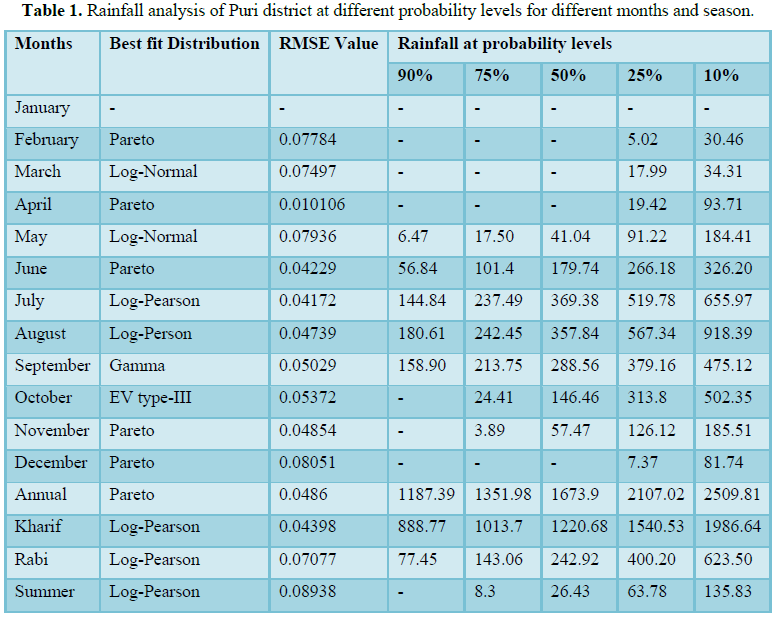
The various parameters like mean, standard deviation, RMSE value, were obtained and noted for different distributions. For generalized extreme value and generalized Pareto distribution the other parameters like shape parameter ξ, scale parameter σ and location parameter µ are also noted for further calculation. Similar procedure is followed for the seasonal, annual and pentad analysis. The rainfall at 90%, 75%, 50%, 25% and 10% probability levels are determined. The distribution “best” fitted to the data is noted down in a tabulated form in Table 1 [7-10].
In the present study, the parameters of distribution for the different distributions have been estimated by FLOOD-flood frequency analysis software. The rainfall data is the input to the software programme. The best fitted distribution of different month and season and annual were presented in Table 1. The annual rainfall in 50% probability was found to be 1673.9 mm for Puri district of Odisha [11-14]. During Kharif at 50% probability level, the rainfall is 1220.68 mm whereas only 242.92 mm and 26.43 mm was received during rabi and summer respectively, so water harvesting structures may be made to grow crops during rabi and summer to utilise the water from the water harvesting structures to increase the cropping intensity of the area. It is also observed that at 75% probability level the June, July, August and September received more than 100 mm, so farmers of these area can grow crops in upland areas suitably paddy can be grown followed by any rabi crop in rabi season like mustard or kulthi in upland areas. In Figure 1, the plot between different months and amount of rainfall in different probabilities were shown, It is observed that July month gets highest amount of rainfall compared to other months [15-17].
CONCLUSION
Forecasting of rainfall is essential for proper planning of crop production. About 70% of cultivable land of Odisha depends on rainfall for crop production. Prediction of rainfall in advance helps to accomplish the agricultural operations in time. It can be concluded that, excess runoff should be harvested for irrigating post-monsoon crops. It becomes highly necessary to provide the farmers with high-yielding variety of crops and such varieties which require less water and are early-maturing in Puri district of Hirakud command area of Odisha. It is also observed that at 75% probability level the June, July, August and September received more than 100 mm, so farmers of these area can grow crops in upland areas suitably paddy can be grown followed by any rabi crop in rabi season like mustard or kulthi in upland areas. Annual rainfall of Puri district is 1673.9 mm at 50% probability level. It is observed that July month gets highest amount of rainfall compared to other months [18].
1. Thom HCS (1966) Some methods of climatological analysis. WMO Technical Note No. 81.
2. Kar G, Singh R, Verma HN (2004) Alternative cropping strategies for assured and efficient crop production in upland rain fed rice areas of eastern India based on rainfall analysis. Agricultural Water Management 67: 47-62.
3. Jat ML, Singh RV, Balyan JK, Jain LK, Sharma RK (2006) Analysis of weekly rainfall for Sorghum based crop planning in Udaipur region. Indian J Dryland Agric Res Dev 21: 114-122.
4. Senapati SC, Sahu AP, Sharma SD (2009) Analysis of meteorological events for crop planning in rain fed uplands. Indian J Soil Cons 37: 85-90.
5. Gumbel EJ (1954) Statistical theory of droughts. Proceedings of ASCE 80: 1-19.
6. Chow VT (1964) Hand book of Applied Hydrology. McGraw Hill Book Co.: New York, pp: 8-28.
7. Biswas BC (1990) Forecasting for agricultural application. Mausam 41: 329-334.
8. Das MK (1992) Analysis of agrometerological data of Bhubaneswar for crop planning. M. Tech. thesis. C.A.E.T., OUAT.
9. Gumbel EJ (1958) Statistics of extremes. Columbia University Press: New York.
10. Harshfield DM, Kohlar MA (1960) An empirical appraisal of the Gumbel extreme procedure. J Geophys Res 65: 1737-1746.
11. Panigrahi B (1998) Probability analysis of short duration rainfall for crop planning in coastal Orissa. Indian J Soil Cons 26: 178-182.
12. Reddy SR (1999) Principles of Agronomy. 1st Edn. Kalyani Publication.
13. Sadhab P (2002) Study of rainfall distributions and determination of drainage coefficient: A case study for coastal belt of Orissa. M. Tech. thesis. C. A. E. T., OUAT.
14. Sharda VN, Das PK (2005) Modeling weekly rainfall data for crop planning in a sub-humid climate of India. Agricultural Water Management 76: 120-138.
15. Subramanya K (1990) Engineering Hydrology. 23rd reprint. Tata Mc-graw Hill Publishing Company Ltd.
16. Subudhi CR (2007) Probability analysis for prediction of annual maximum daily rainfall of Chakapada block of Kandhamal district of Orissa. Indian J Soil Cons 35: 84-85.
17. Subudhi CR, Suryavansi S, Jena N (2019) Rainfall probability analysis for crop planning in Anugul block of Anugul district of Hirakud command area of Odisha, India. Int J Human Soc Sci 8: 49-54.
18. Weibull W (1951) A statistical distribution functions of wide applicability. J Appl Mech Tran ASME 18: 293-297.
-
 Table 1
QUICK LINKS
- SUBMIT MANUSCRIPT
- RECOMMEND THE JOURNAL
-
SUBSCRIBE FOR ALERTS
RELATED JOURNALS
- Journal of Biochemistry and Molecular Medicine (ISSN:2641-6948)
- Proteomics and Bioinformatics (ISSN:2641-7561)
- Journal of Genetics and Cell Biology (ISSN:2639-3360)
- Journal of Womens Health and Safety Research (ISSN:2577-1388)
- Journal of Genomic Medicine and Pharmacogenomics (ISSN:2474-4670)
- Food and Nutrition-Current Research (ISSN:2638-1095)
- Advances in Nanomedicine and Nanotechnology Research (ISSN: 2688-5476)